Tutorials

I plan to create some tutorials and post them on this page. I have completed five so far.
:

Delay Line With Loss
Feedback Delay Networks
Schroeder Reverberators
Simple State Space Filter
Multiport Networks

I have implemented some of the concepts described in these tutorials as C++ classes. C++ code and documentation are available here.

Delay Line With Loss

Sample delays are an important component of several reverb algorithms. I like to think of a sample delay as a propagation delay that can also introduce loss and frequency shaping. Thus I define my lossy delay line with the following transfer function:

$h(z)=\frac{gz^{-N}}{1-dz^{-1}}$

where N is the sample delay and g and d, which I call gain and damping, respectively, are parameters of a simple low-pass filter. The corresponding difference equation is

$y(n)=dy(n-1)+gx(n-N)$

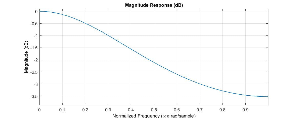
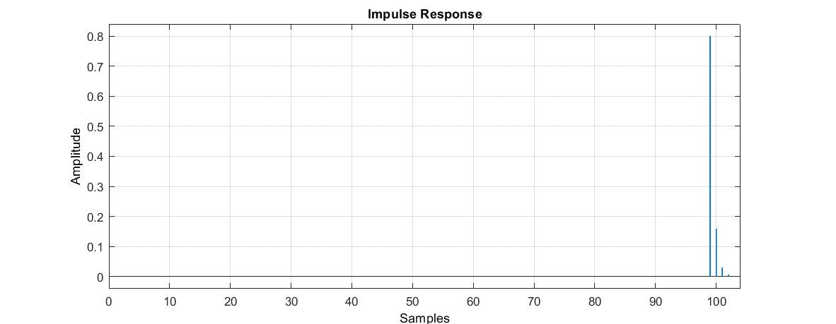
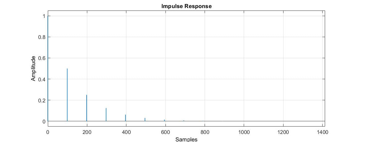
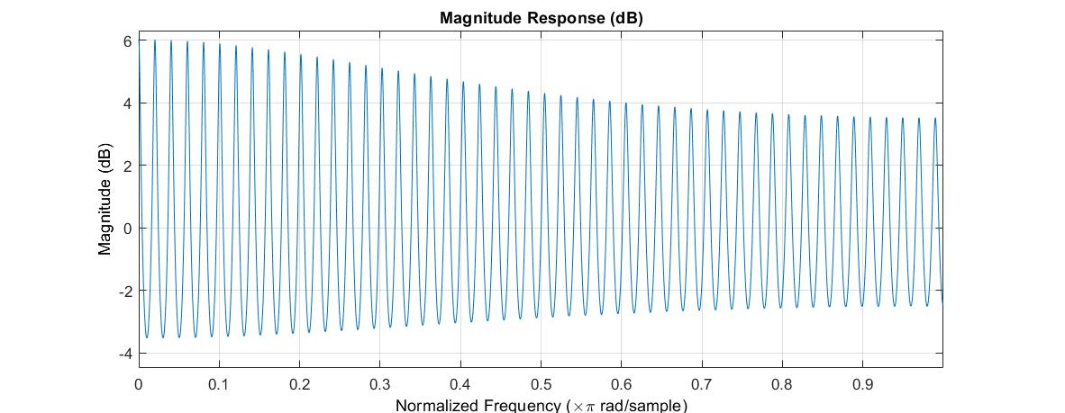
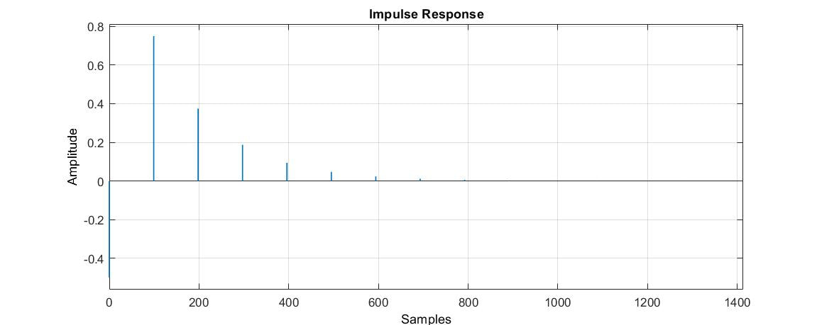
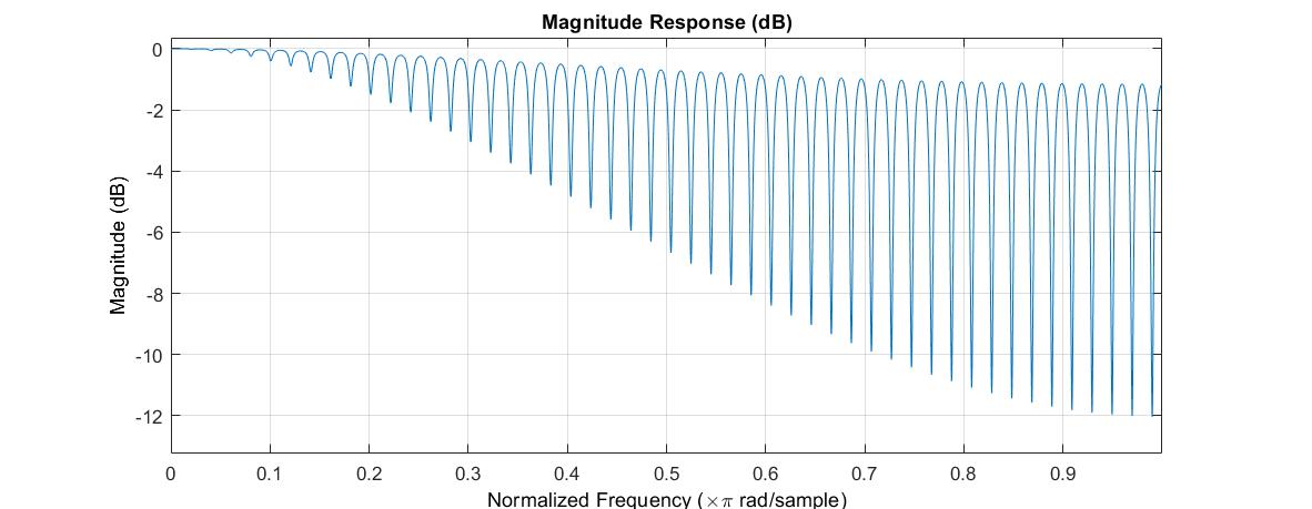
The magnitude of the frequency response and the impulse response are shown below.

The magnitude of the frequency response varies between a low frequency maximum and a high frequency minimum given by

$\begin{align} H(0)&=\frac{g}{1-d} \notag \\ H(f_s)&=\frac{g}{1+d} \notag \end{align}$

For a path of length L, I will assume that the magnitude of the frequency response is given by

$H(f)=10^{-A(f)L/20}$

where A(f) is the frequency-dependent absorption coefficient in dB/m. Since this coefficient varies by orders of magnitude over the range of audible frequencies (see, for example, here), I will assume that A(0) = 0 and let A be the value of A(f) at the Nyquist frequency. Then we have

$\begin{align} 1&=\frac{g}{1-d} \notag \\ 10^{-AL/20}&=\frac{g}{1+d} \notag \end{align}$

so that

$\begin{align} d&=\frac{1-10^{-AL/20}}{1+10^{-AL/20}} \notag \\ g&=1-d \notag \end{align}$

The sample delay N also depends on the path length L, the sampling frequency f_s, and the speed of sound, c.

$N=\mathrm{round}(Lf_s/c)$

Thus we specify a lossy delay line to model a propagation path of length L (m) with high frequency absorption coefficient A (dB/m).

C++ Implementation

The implementation files Delayline.h and Delayline.cpp are included here.

Feedback Delay Networks

Feedback delay networks (FDN) can be used to create a reverb effect for an audio signal. This tutorial shows that a FDN can be viewed as a generalization of a classic state space filter. It also examines a specific type of FDN and provides suggestions for C++ implementation.

Introduction

A discrete time, linear, time-invariant system (LTIS) can be represented by the following equations:

$\begin{align} \mathbf{x}(n+1)&=\mathbf{Ax}(n)+\mathbf{B}u(n) \notag \\ y(n)&=\mathbf{Cx}(n)+Du(n) \notag \end{align}$

where u(n) is the single input, y(n) is the single output, and x(n) is a vector of state variables. A is a N by N state transition matrix (N is the number of state variables), B is a column vector (N rows), and C is a row vector (N columns). D is a scalar value, which, for simplicity, is assumed to be zero.

Upon application of the z transform, the state space filter looks like this:

$\begin{align} z\mathbf{x}(z)&=\mathbf{Ax}(z)+\mathbf{B}u(z) \notag \\ y(z)&=\mathbf{Cx}(z) \notag \end{align}$

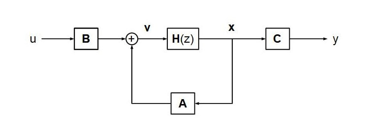
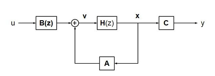
These equations can be represented by a block diagram:

To turn this structure into a FDN, replace the one sample delay with a more general transform H(z) as shown below.

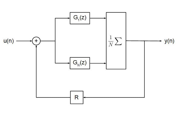
For example, instead of a one sample delay, H(z) can represent a bank of delay lines with different delays, i.e.,

$\mathbf{H}(z)=\begin{bmatrix} z^{-M_1} & 0 & \cdots & 0 \\ 0 & z^{-M_2} & \cdots & 0 \\ \vdots & \vdots & \ddots & \vdots \\ 0 & 0 & \cdots & z^{-M_N} \end{bmatrix}$

In the time domain, this is equivalent to

$x_k(n)=v_k(n-M_k)$

H(z) can also represent a bank of lossy delay lines as defined in the previous tutorial.

$\mathbf{H}(z)=\begin{bmatrix} \frac{g_1z^{-M_1}}{1-d_1z^{-1}} & 0 & \cdots & 0 \\ 0 & \frac{g_2z^{-M_2}}{1-d_2z^{-1}} & \cdots & 0 \\ \vdots & \vdots & \ddots & \vdots \\ 0 & 0 & \cdots & \frac{g_Nz^{-M_N}}{1-d_Nz^{-1}} \end{bmatrix}$

which is equivalent to

$x_k(n)=d_kx_k(n-1)+g_kv_k(n-M_k)$

As discussed in the previous tutorial, the sample delays as well as the g and d parameters can be determined from path lengths and the high frequency absorption coefficient. We will address the topic of path lengths later in this tutorial.

Choosing the State Transition Matrix and Associated Vectors

This section edited on February 6, 2021 to introduce a change in the feedback matrix.

The A, B, and C parameters are chosen as follows:

$\begin{align} \mathbf{A}&=\frac{R}{N}\mathbf{O}-\mathbf{I}\notag\\ \mathbf{B}&=\begin{bmatrix} 1 \\ 1 \\ \vdots \\ 1 \end{bmatrix}\notag\\ \mathbf{C}&=\begin{bmatrix}1&1&\cdots&1 \end{bmatrix}\notag \end{align}$

where O is a N by N matrix of ones and 0 <= R < 2. The parameter R affects the impulse response of the FDN and can be made available as a user parameter. For R = 2, the FDN teeters on the edge of stability and for R > 2, it is definitely unstable!

This choice leads to considerable simplification of the system. First of all, the output is simply the average of the components of the state variable.

$y(n)=\frac{1}{N}\sum_{k=1}^Nx_k(n)$

The input to the k-th delay line is given by

$\begin{align} v_k(n)&=u(n)+\frac{R}{N}\sum_{l=1}^Nx_l(n)-x_k(n)\notag\\ &=u(n)+Ry(n)-x_k(n)\notag \end{align}$

Thus the vector v(n) is given by

$\mathbf{v}(n)=\mathbf{B}[u(n)+Ry(n)]-\mathbf{x}(n)$

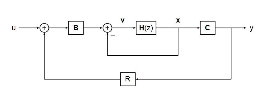
This leads to the following block diagram:

We can also display the FDN without vector notation:

where

$\large \begin{align} G_k(z)&=\frac{H_k(z)}{1+H_k(z)}\notag\\ &=\frac{g_kz^{-M_k}}{1-d_kz^{-1}+g_kz^{-M_k}}\notag \end{align}$

Choosing Path Lengths

The path lengths represent various propagation paths that may exist in the "room", i.e., the reverberant space being modeled by the FDN. For my version of the FDN, I determine N path lengths varying exponentially from a maximum to a minimum. The maximum is the room length, which I derive from the room area (a popular user input) assuming the floor of the room is a golden rectangle. The minimum path is one tenth the maximum. I have not performed any comparisons of this with other methods. You are welcome to experiment!

Summary of Calculations

Choose an "order" N. It does not have to be very high - N = 6 works fine for me.
Determine a set of N path lengths based on the room area (user input) as just discussed.
Determine the N sample delays and gain and damping values based on the path lengths and the high frequency absorption coefficient (user input)

At this point the FDN is fully specified and ready to process audio samples. The state vector x is initially all zeros. Each audio sample processing step includes the following:

Compute the output of each of the filters Gk(z), using the current FDN input and previous FDN output as inputs.
The next output is the average of the filter outputs.

The filters can be implemented as instances of a C++ class, with methods to set the filter parameters and a method to process one or more samples.

Extension of the FDN Reverb

A more elaborate FDN can be created by replacing the simple vector of ones B with a more general vector B(z) as in the figure below.

For example, B(z) may be given by

$\mathbf{B}(z)=\mathbf{H}_d\mathbf{D}(z)\mathbf{o}$

where o is a column vector of ones, D(z) is a bank of delays similar to H(z), and H is a Hadamard matrix (please excuse the confusing notation). This structure is an example of what is sometimes called a diffuser and provides a more interesting input to the feedback loop than the FDN described earlier.

The Hadamard matrix is a square matrix whose elements are either +1 or -1 and whose order is either 1, 2, or a multiple of 4. The output of the delay bank is a vector of delayed versions of the scalar input with different delays and the output of the Hadamard operation is a vector of sums and differences of these delayed inputs. In simple terms, the diffuser mixes things up a bit ahead of the feedback loop.

If A and C are still defined as in the FDN described earlier, the complete system looks like this:

In this figure, the thin arrows represent scalar values and the thick arrows represent vectors. The blank box simply expands the scalar input u into a vector of copies of u. DDB is the diffuser delay bank and FDB is the FDN delay bank (previously known as H(z)). H is the hadamard matrix and the box labeled R expands the scalar output y into a vector of copies of y multiplied by the "reflectance" R.

The following set of difference equations describes the operation of this system:

$\begin{align*} y(n)&=\frac{1}{N}\sum_{k=1}^Nx_k(n) \\ \mathbf{v}_1(n)&=\begin{bmatrix} u(n-D_1) \\ \vdots\\ u(n-D_N) \end{bmatrix} \\ \mathbf{v}_2(n)&=\mathbf{Hv}_1(n)+\mathbf{R}y(n)-\mathbf{x}(n) \\ \mathbf{x}(n)&=\begin{bmatrix} v_{21}(n-F_1)\\ \vdots\\ v_{2N}(n-F_N) \end{bmatrix} \end{align*}$

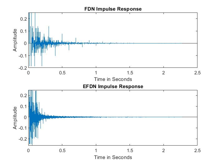
The figure below compares the impulse response of the more basic FDN described earlier and this "enhanced" FDN with similar delay values. In this example, the DDB delays are significantly larger than the FDB delays. Other examples, not shown here, indicate that the result varies significantly with delay values. Some experiments with an audio plug-in based on the EFDN show that it is livelier than the basic FDN.

Schroeder Reverberators

The subject of artificial reverberation was initiated in the early 1960s by Manfred Schroeder and Ben Logan(ref). They and others used various combinations of comb filters and all pass filters to add a reverb effect to an audio signal. This tutorial provides an overview of what I will call Schroeder reverb and discuss my own implementation in more detail.

We begin with a review of comb and all pass filters.

Comb Filter

The basic feedforward comb filter is defined by the following difference equation

$y(n)=x(n)+R x(n-N)$

The transfer function for this filter is given by

$h(z)=1+Rz^{-N}$

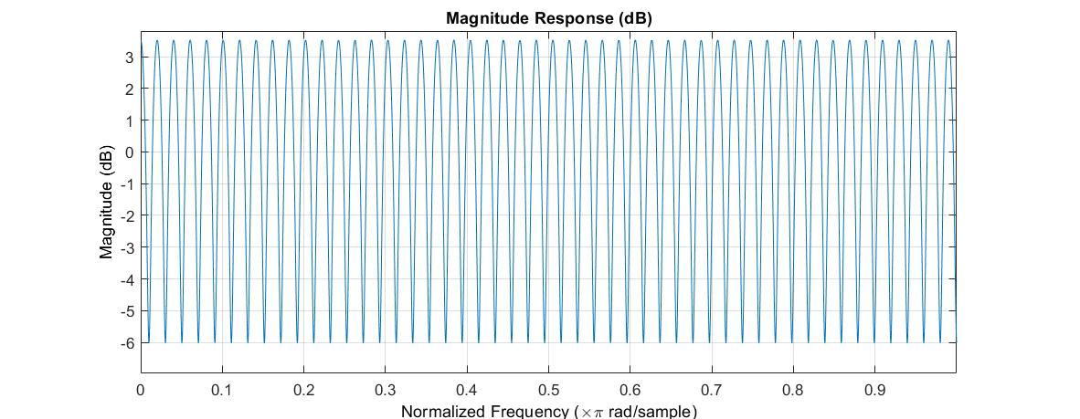
The magnitude of the frequency response looks like a comb!

The impulse response of the feedforward comb filter is not very interesting, consisting only of the original impulse and a single echo. The feedback comb filter, given by the following difference equation and transfer function, offers a bit more.

$\begin{align} y(n)&=x(n)+Ry(n-N) \notag \\ h(z)&=\frac{1}{1-Rz^{-N}} \notag \end{align}$

While the frequency response still looks like a comb, the impulse response of the feedback comb filter is a series of echos.

Note that the absolute value of R must be less than 1 to insure stability.

The feedback comb filter can be viewed as a rough model of a sound wave being reflected back and forth between two walls. The sample delay N models the propagation delay and the factor R models the loss due to absorption by the walls. We can extend the model by replacing the sample delay with a lossy delay line. This leads to a low-pass feedback comb filter with a transfer function given by

$\begin{align} h(z)&=\frac{1}{1-R\frac{g}{1-dz^{-1}} z^{-N}} \notag \\ &=\frac{1-dz^{-1}}{1-dz^{-1}+Rgz^{-N}} \notag \end{align}$

This formulation attempts to separate the loss due partial reflection at the walls (R) and the loss during propagation (g and d). We can compute N, g, and d from a path length and high frequency absorption coefficient as discussed in a previous tutorial. Again, R must be less than 1 to maintain stability.

The difference equation for the low pass feedback comb filter is given by

$y(n)=dy(n-1)+gR y(n-N)+x(n)-dx(n-1)$

This can also be written in a simple state variable form:

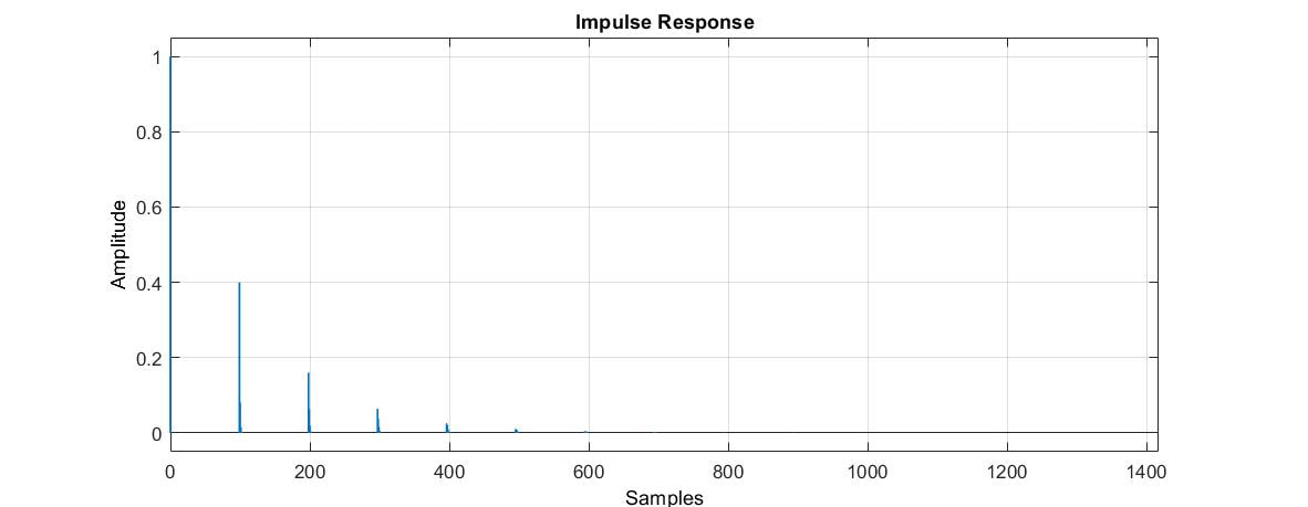
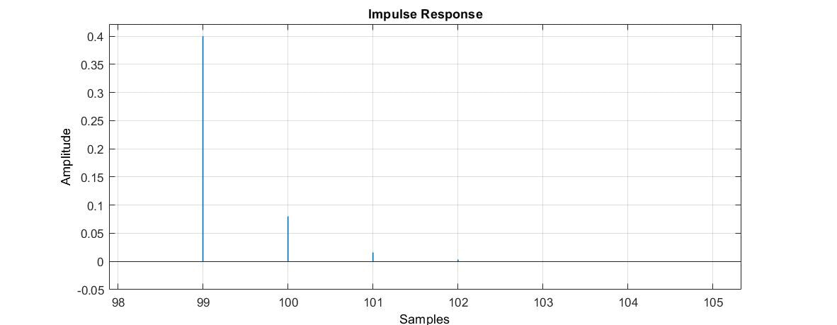
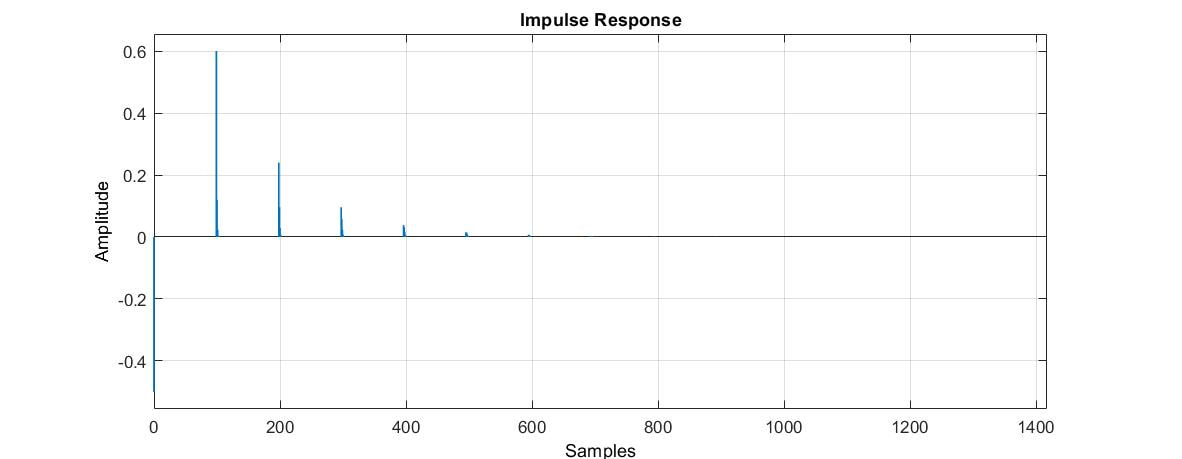
$\begin{align} s(n)&=ds(n-1)+gRy(n-N) \notag \\ y(n)&=s(n)+x(n) \notag \end{align}$

The frequency response of the low pass feedback comb filter still looks like a comb, but has a low pass envelope. The impulse response is similar to the basic feedback comb filter, but a closer look at one of the echos reveals additional echos, giving the primary echo a bit more duration.

The Schroeder reverb described later on uses a bank of low pass feedback comb filters.

All Pass Filter

The difference equation and transfer function for the basic all pass filter are

$\begin{align} y(n)&=-Rx(n)+x(n-N)+Ry(n-N) \notag \\ h(z)&=\frac{-R+z^{-N}}{1-R z^{-N}} \notag \end{align}$

The magnitude of h(z) is 1 for all frequencies, hence the name of the filter. The impulse response is a series of echos.

Once again, we can replace the sample delay with a lossy delay line. The transfer function becomes.

$\begin{align} h(z)&=\frac{-R+\frac{g}{1-dz^{-1}}z^{-N}}{1-R\frac{g}{1-dz^{-1}}z^{-N}} \notag \\ &=\frac{-R+Rdz^{-1}+gz^{-N}}{1-dz^{-1}-R gz^{-N}} \notag \end{align}$

With this modification the filter is no longer all pass. The magnitude of the frequency response looks like this:

The impulse response is similar to that of the basic all pass filter, but includes secondary echos, like the low pass feedback comb filter

In spite of the contradiction, I call this the low pass all pass filter.

C++ code for both the low pass comb filter and the low pass all pass filter is available here.

A Schroeder Reverb Design

There is a popular Schroeder reverb called Freeverb developed by "Jezar at Dreampoint". Freeverb consists of a bank of 8 low pass feedback comb filters followed by a cascade of 4 all pass filters so that the overall transfer function is

$h(z)=\left(\sum_{k=1}^8\mathrm{CF}_k(z) \right )\prod_{k=1}^4\mathrm{APF}_k(z)$

The all pass filters in Freeverb have the following transfer function:

$h(z)=\frac{-1+(1+R)z^{-N}}{1-Rz^{-N}}$

This variation is all pass only for a particular value of R. The parameters of the filters, including sample delays, were all apparently chosen by Jezar and seem to provide a good reverb effect.

For my implementation, I have chosen to use the same overall structure of a bank of 8 low pass feedback comb filters followed by a chain of 4 all pass filters. However, my version uses the low pass all pass filter. The sample delay N and the g and d parameters of each filter are computed from a path length L (meters), a high frequency absorption coefficient A (dB/meter), and the sampling frequency f_s, as previously described.

The path lengths for the filters are determine in the same way as for the FDN, i.e., a sequence of lengths starting from a maximum length, based on the room area and geometric assumptions, and decreasing exponentially to a minimum length.

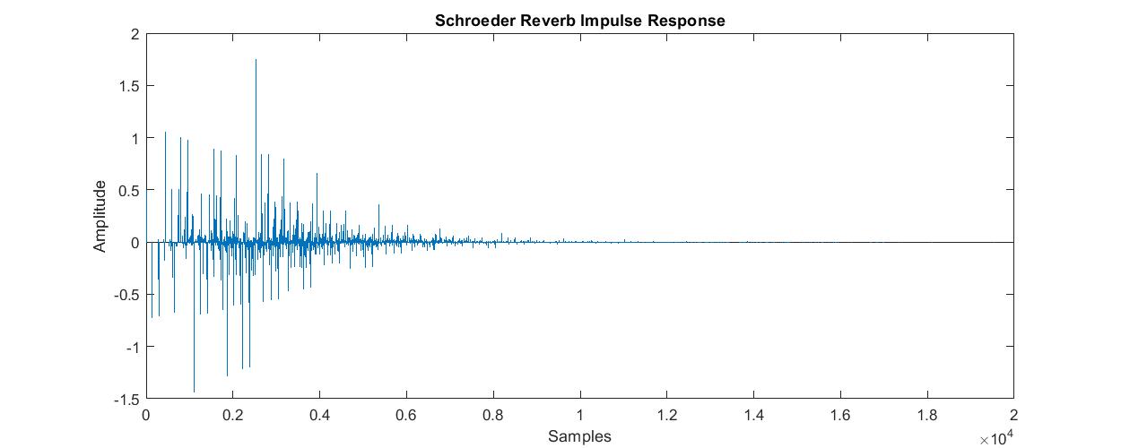
Here is an example of the impulse response of this Schroeder reverb

I have implemented this design as a VST audio plugin for Windows 64 and 32 bit. You can download a copy of the plugin from my audio plugin page.

Simple State Space Filter

This tutorial describes a popular state space filter that is also described in my book. It can be used as either a low-pass, high-pass, or band-pass filter. It is computationally efficient and I have used it in my wah-wah plugin.

The filter is defined by the following set of equations:

$\begin{align} x_H(n+1)&=-x_L(n)-Dx_M(n)+u(n) \notag \\ x_M(n+1)&=x_M(n)+F_1x_H(n+1) \notag \\ x_L(n+1)&=x_L(n)+F_1x_M(n+1) \notag \end{align}$

Applying the z transform, we have

$\begin{align} zx_H(z)&=-x_L(z)-Dx_M(z)+u(z) \notag \\ zx_M(z)&=x_M(z)+zF_1z_H(z) \notag \\ zx_L(z)&=x_L(z)+zF_1z_M(z) \notag \end{align}$

where D is another sort of damping factor and F_1 is given by

$F_1=2\sin(\pi f_c/f_s)$

where f_c is a center or cut-off frequency and f_s is the sampling frequency.

From this it is straightforward to determine that

$\begin{align} \frac{x_H(z)}{u(z)}&=\frac{1-2z^{-1}+z^{-2}}{A(z)} \notag \\ \frac{x_M(z)}{u(z)}&=\frac{F_1(1-z^{-1})}{A(z)} \notag \\ \frac{x_L(z)}{u(z)}&=\frac{F_1^2}{A(z)} \notag \end{align}$

where

$A(z)=1+(DF_1+F_1^2-2)z^{-1}+(1-DF_1)z^{-2}$

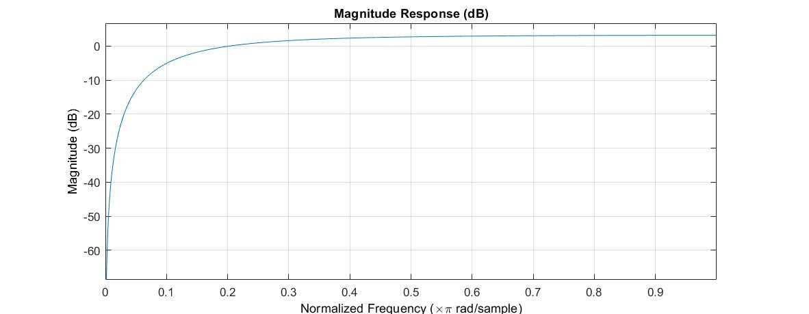
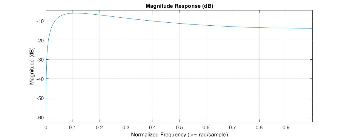
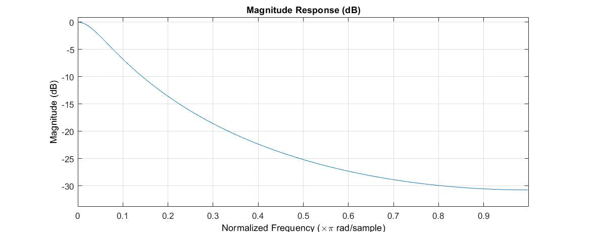
I have excluded a common factor of z since it only introduces a one sample delay. Plots of the magnitudes of the frequency responses of these transfer functions show that the filter provides a high-pass, band-pass, and low-pass output.

C++ code for the filter is available here.

Multiport Networks

A few years ago (2013 to be exact) I published a paper in the AES Journal on something I called multiport acoustic elements. If you are a member of AES, you can access the paper here. A multiport acoustic element represents an acoustic entity that has two or more interface ports, each with an incoming and outgoing acoustic wave. My paper describes three such elements:

Waveguide - Represents a medium that supports propagation of plane acoustic waves. Bidirectional. Characterized by a time delay and attenuation.
Junction - A connection among the ends of two or more waveguides.
Reflector - A termination of or discontinuity in a waveguide. Characterized by a reflection coefficient.

The waveguide and reflector are two-port elements; the junction usually has three or more ports.

The inputs and outputs at the ports of the elements are acoustic pressure waves and the relations between the inputs and outputs are determined by assumptions about the behavior of the elements and the properties of acoustic plane waves. Recently I have been developing a set of audio signal processing elements based on these acoustic elements. The input and output audio signal processing element port are audio sample sequences rather than acoustic plane waves.

For the waveguide element, I simply use a pair of delay lines with loss as described in the first tutorial. The relation among the port inputs and outputs is given by:

$\begin{align*} y_0(n)&=dy_0(n-1)+(1-d)x_1(n-N)) \\ y_1(n)&=dy_1(n-1)+(1-d)x_0(n-N)) \end{align*}$

where x is a port input, y is a port output, and the subscript is the index of the port. The damping d and sample delay N are determined just as they are for the delay line.

The junction model is based on an idealized connection of the ends of two or more waveguides with the same acoustic impedance. The input/output relation is given by

${\color{Black} y_p(n)=\frac{2}{P}\sum_{q=0}^Px_q(n)-x_p(n) }$

where P is the number of ports in the junction.

The reflector represents a waveguide termination or a connection between two waveguides with different acoustic impedance. The input/output relation is given by

${\color{Black} \begin{align*} y_0(n)&=\Gamma x_0(n)+(1-\Gamma)x_1(n) \\ y_1(n)&=(1+\Gamma)x_0(n)-\Gamma x_1(n) \end{align*} }$

where Gamma is a reflection coefficient ranging between -1 and +1.

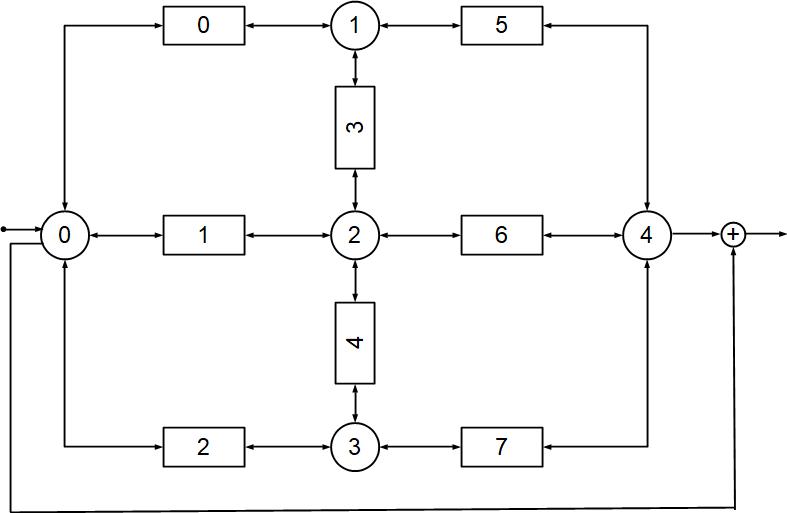
I have coded a simple C++ class hierarchy consisting of a base class called MuitiPort and three derived classes called WaveGuide, Junction, and Reflector. The port inputs and outputs are implemented as shared pointers so that the elements can easily be connected to one another to create a network. An example of such a network is shown below.

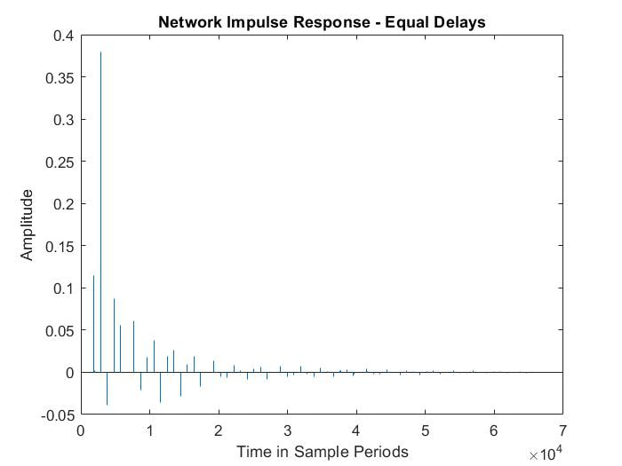
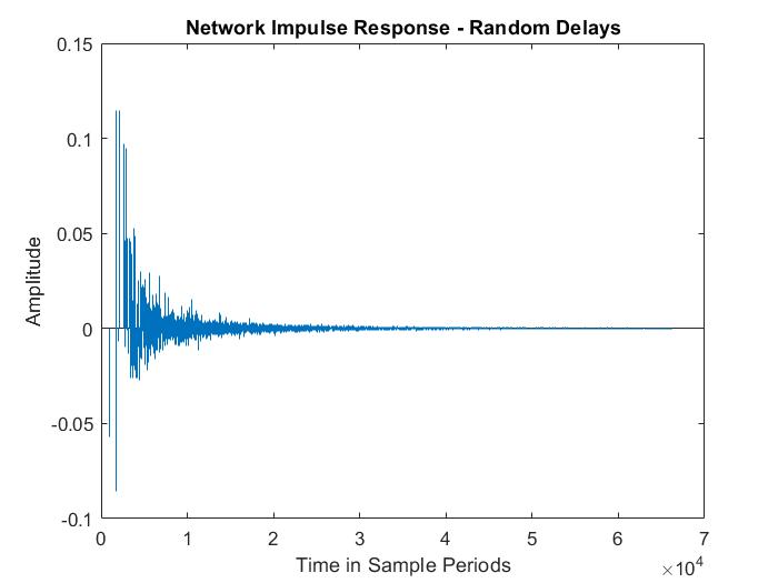
The network contains five junctions, indicated by the circles and numbered from 0 to 4, and eight waveguides, indicated by the rectangles and numbered from 0 to 7. This network is set up to process an audio input on the west port of junction 0. The audio output is the sum of the outputs of the west port of junction 0 and the east port of junction 4. The two figures below display the impulse response of this network. For the figure to the left, the waveguide sample delays were all set to the same value. The resulting response is a series of evenly spaced echoes. For the figure to the right, the delays were randomized. This results in a response that corresponds to a reverb effect!

To facilitate construction of a network, I have coded a class called MPnetwork that has methods for adding and interconnecting network elements.

I have coded a plugin called Netverb based on this network. You may obtain a copy (Windows only) from my Audio Plugins page. C++ code for the multiport network elements is available here.