Besides audio signal processing, I have an ongoing interest in the field of statistical pattern recognition with particular emphasis on feature extraction and clustering. Although I may move this topic to another domain in the future, I will use this site to get started.
Clustering
During my graduate studies at Purdue University, Ken Fukunaga (my major professor) and I developed some new approaches to clustering, which I will define as organizing a set of observations into groups based on some kind of logic or criterion. Shortly after completing my studies, I came up with yet another algorithm, which I shared with Ken and P. M. Narendra, one of his students. We published the algorithm in 1976 (paper). By then my career had taken me in other directions and I have not been active in the field until recently. I will be sharing my current work on this page.
Brief Description of the Algorithm
The algorithm is described in detail in the original paper, so this is only a brief overview.
We start with a set of N observations and a metric of the distance between any two objects. We select a threshold distance and consider two
observations to be neighbors if the distance between them is less than or equal to the threshold value. We can then construct a graph where
each observation becomes a node (or vertex) and there is a edge from each node to each of its neighbors (no more than one edge per node
pair). The degree of each node, i.e., the number of edges connected to the node, is equal to the number of neighbors of that node. It is also a
crude measure of the local density of observations.
Once the graph is established, we can determine a parent node for each node. For a given node, the parent node is the node in its
neighborhood, which includes the node itself and all of its neighbors, with the largest number of neighbors. We resolve ties arbitrarily,
but consistently, based on the index of the node. If the node itself is selected, it is an orphan and also the root of a cluster.
Having identified parent nodes for every node, we then assign a unique cluster ID to each orphan. The cluster IDs of the remaining nodes are
determined recursively using the rule ”your cluster ID is that of your parent”.
MATLAB Implementation
My MATLAB implementation of the algorithm is a MATLAB function that makes use of the MATLAB graph object. The input to the function is an observation matrix X that represents the observations to be clustered and a distance threshold r. Each row of the matrix X represents an observation and each column represents a numerical attribute of the object. The distance between two objects is currently based on the Euclidean metric, but this can easily be modified.
To create the graph object, we start by creating an empty graph and use the addnode method to create as many nodes as there are objects.
G = graph;
G = addnode(G,N);
We then use the addedge method to add the edges one at a time based on the distance threshold.
for i=2:N
for j=1:i-1
if (sum((X(i,:)-X(j,:)).^2)<=r2)
G = addedge(G,i,j);
end
end
end
The nested loop covers all unique pairs of observations. The square of the distance threshold, r2, is used for convenience.
Now we are ready to find the parent of each object - the neighbor with the most neighbors. The degree method generates a vector of the number of neighbors for each node
nbrs=degree(G);
Moreover, the neighbors method provides a list of the neighbors of each node. This makes it easy to determine the parents.
for n=1:N
for m=neighbors(G,n)'
if (nbrs(m)>nbrs(pnode(n))) ||...
((nbrs(m)==nbrs(pnode(n)))&&m>pnode(n))
pnode(n)=m;
end
end
end
The parents are stored in the vector pnode, which is initialized as
pnode = 1:N;
that is, each node starts out as an orphan. Note the simple, but consistent tie-breaking rule.
Once the parents are determined, the rest is easy. Each orphan becomes the root of a cluster and the remaining objects are assigned recursively to their parent's cluster. The previous code can be expanded to establish the roots
M=0;
cls=zeros(N,1);
for n=1:N
for m=neighbors(G,n)'
if (nbrs(m)>nbrs(pnode(n))) ||...
((nbrs(m)==nbrs(pnode(n)))&&m>pnode(n))
pnode(n)=m;
end
end
if pnode(n)==n
M=M+1;
cls(n)=M;
end
end
Finally, the recursive part.
for n=1:N
pn=n;
while cls(pn)==0
pn=pnode(pn);
end
cls(n)=cls(pn);
end
The complete code for this function is available from MATLAB Central.
C++ Version
The algorithm is also easy to code in C++. The C++ standard library does not appear to include a graph class, but you can simply use a vector of vectors to establish a simple graph.
std::vector<std::vector<std::size_t>> graph;
Each element of the outer vector graph represents an observation and each element of the inner vector is the index of a neighboring observation. The graph is constructed by first setting the size of the outer vector
graph.resize(N);
and then, for each pair of observations nearer to each other than the threshold distance
graph[n].push_back[m];
graph[m].push_back[n];
Once the graph is constructed, the neighbor counts are given by
nbrs[n] = graph[n].size();
and you can iterate through the neighbors using a for-range loop
for (auto nbr : graph[n])
The complete C++ code for the algorithm, coded as a C++ function, is located here.
Qt C++ Application
I have implemented the algorithm as a C++ Windows application using Qt Creator. I have not yet deployed the application, but I can run it in the Qt Creator environment. The current functionality includes the following:
The next sections describe the application of Clusterizer to some publicly available data sets.
Anuran Calls Data Set - Eng. Juan Gabriel Colonna et al., Universidade Federal do Amazonas
The data set consists of 7195 observations derived from recordings of frog calls, with 22 real number valued attributes for each observation. The researchers describe the data set as follows:
"This dataset was used in several classifications tasks related to the challenge of anuran species recognition through their calls. It is a multilabel dataset with three columns of labels. This dataset was created segmenting 60 audio records belonging to 4 different families, 8 genus, and 10 species. Each audio corresponds to one specimen (an individual frog), the record ID is also included as an extra column. We used the spectral entropy and a binary cluster method to detect audio frames belonging to each syllable. The segmentation and feature extraction were carried out in Matlab. After the segmentation we got 7195 syllables, which became instances for train and test the classifier. These records were collected in situ under real noise conditions (the background sound). Some species are from the campus of Federal University of Amazonas, Manaus, others from Mata Atlântica, Brazil, and one of them from Cardoba, Argentina. The recordings were stored in wav format with 44.1kHz of sampling frequency and 32bit of resolution, which allows us to analyze signals up to 22kHz. From every extracted syllable 22 MFCCs were calculated by using 44 triangular filters. These coefficients were normalized between -1 and 1."
MFCC stands for Mel Frequency Cepstrum Coefficient and is popular in the speech recognition arena.
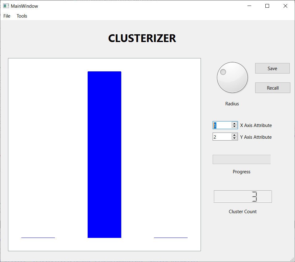
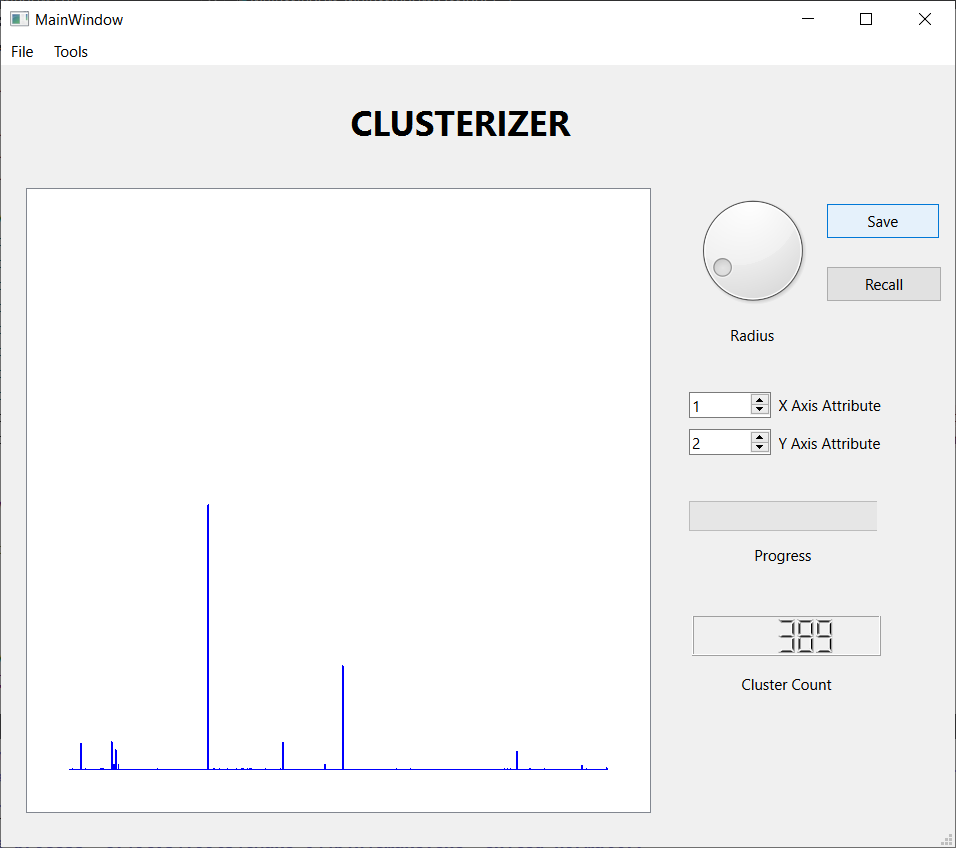
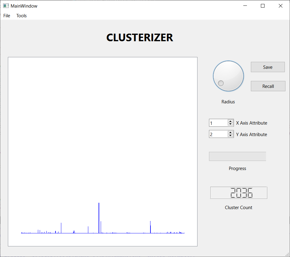
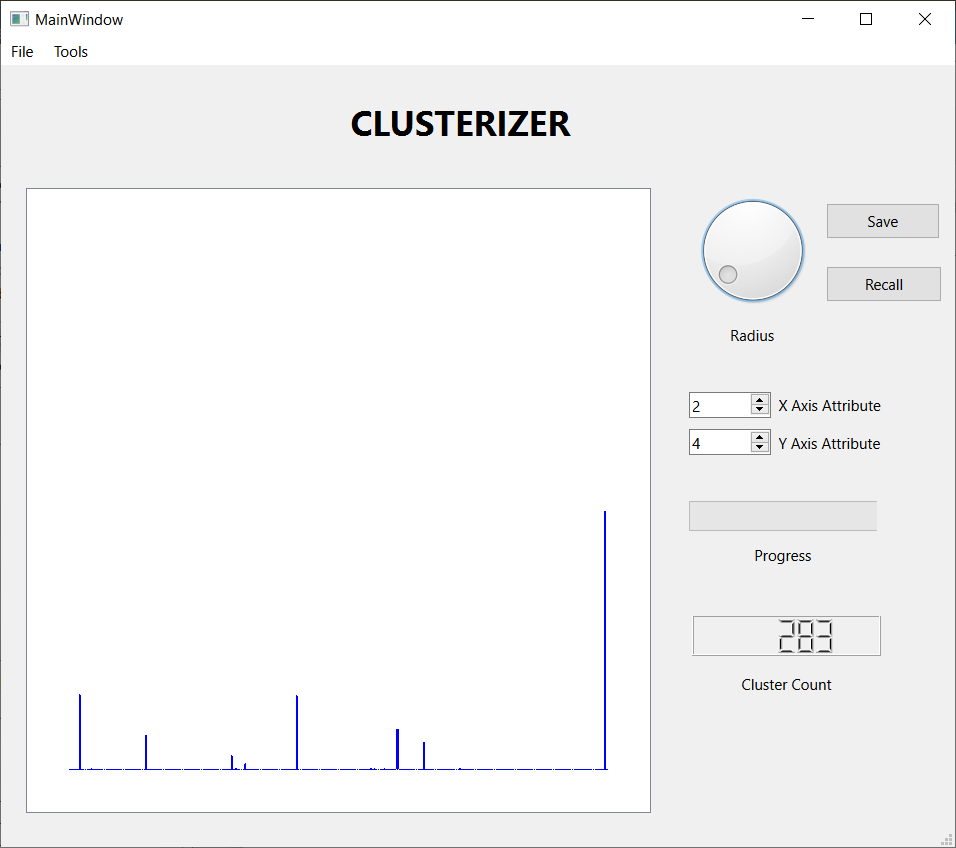
I reformatted the data set into a 7195 by 22 .csv file and processed it with Clusterizer. The first step is to read in the data set and compute the minimum and maximum inter-observation distance. This required less than one minute using an aging Dell laptop running Windows 10. Each run of the clustering algorithm also required a little less that one minute. I used the histogram feature to guide adjusting the threshold distance. The following figures show the results of three runs.
- Select and read a .csv file of observations and attributes. Each line of data contains a comma separated list of the attributes of one observation. The attributes are assumed to be real numbers.
- Select the threshold distance that determines whether or not two observations are neighbors. The threshold distance can be varied from the smallest to the largest inter-observation distance. There is a limited ability to save and recall a threshold value.
- Run the clustering algorithm.
- Display a scatter plot of two selected attributes of the observations. If the clustering algorithm has been run, each cluster will have a unique color on the plot.
- Display a histogram of the cluster populations.
- Write the results of the clustering algorithm to a file for further analysis, perhaps with MATLAB.
The next sections describe the application of Clusterizer to some publicly available data sets.
Anuran Calls Data Set - Eng. Juan Gabriel Colonna et al., Universidade Federal do Amazonas
The data set consists of 7195 observations derived from recordings of frog calls, with 22 real number valued attributes for each observation. The researchers describe the data set as follows:
"This dataset was used in several classifications tasks related to the challenge of anuran species recognition through their calls. It is a multilabel dataset with three columns of labels. This dataset was created segmenting 60 audio records belonging to 4 different families, 8 genus, and 10 species. Each audio corresponds to one specimen (an individual frog), the record ID is also included as an extra column. We used the spectral entropy and a binary cluster method to detect audio frames belonging to each syllable. The segmentation and feature extraction were carried out in Matlab. After the segmentation we got 7195 syllables, which became instances for train and test the classifier. These records were collected in situ under real noise conditions (the background sound). Some species are from the campus of Federal University of Amazonas, Manaus, others from Mata Atlântica, Brazil, and one of them from Cardoba, Argentina. The recordings were stored in wav format with 44.1kHz of sampling frequency and 32bit of resolution, which allows us to analyze signals up to 22kHz. From every extracted syllable 22 MFCCs were calculated by using 44 triangular filters. These coefficients were normalized between -1 and 1."
MFCC stands for Mel Frequency Cepstrum Coefficient and is popular in the speech recognition arena.
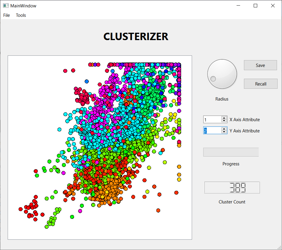
I reformatted the data set into a 7195 by 22 .csv file and processed it with Clusterizer. The first step is to read in the data set and compute the minimum and maximum inter-observation distance. This required less than one minute using an aging Dell laptop running Windows 10. Each run of the clustering algorithm also required a little less that one minute. I used the histogram feature to guide adjusting the threshold distance. The following figures show the results of three runs.
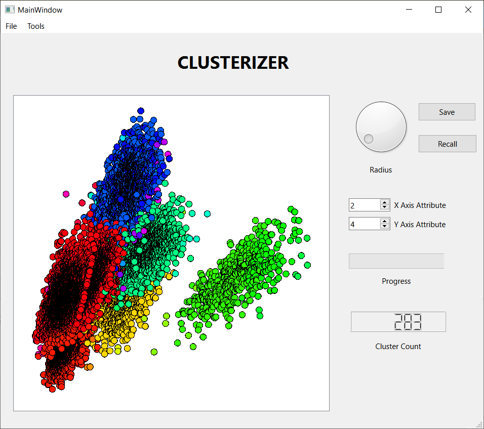
These three screen shots show the histograms for three successively smaller values of the threshold distance. When the threshold is large, nearly every observation lands in one large cluster, not a very satisfying result. Reducing the threshold, we get a more interesting result, with several sizable clusters along with a few hundred outliers. Reducing the threshold further, we get over 2000 tiny clusters along with a dozen or so clusters with notable populations. Which is the best result? I don't know, but I liked the middle one best, so I saved the results for further analysis. I also looked at some scatter plots using a few attribute pairs. I have included an example
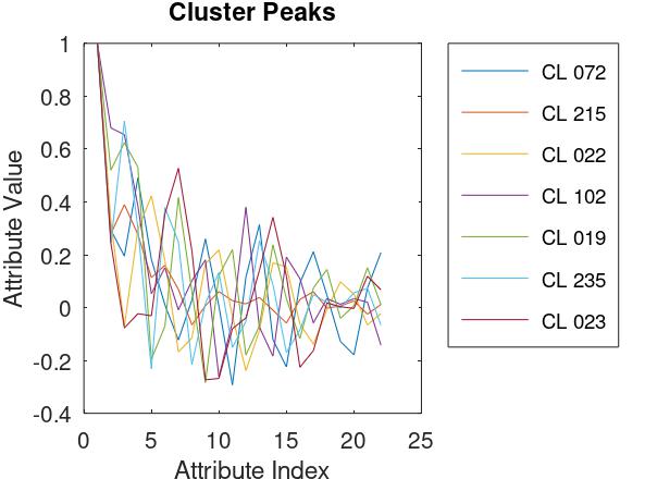
The Save Data feature of Clusterizer creates a .csv file listing the IDs (i.e., indices) of the cluster and the parent of each observation. Using a GNU Octave script (I no longer have access to MATLAB), I determined the size (i.e., number of observations) of each cluster, sorted the clusters according to population, and determined the "top 95", i.e., the smallest subset of clusters containing 95% of the observations. The "Cluster Peaks" plot shows, for each of the 7 clusters in the top 95, the attribute values of the "orphan" that establishes the cluster.
Using another Octave script, I generated the following table. Columns 2 - 8 correspond to the 7 "top 95" clusters (cluster ID 72, 215, ...). The first column indicates the family, genus, and species of the recorded frog. This data was provided to support a "supervised learning" algorithm and was not used for clustering, which is "unsupervised". Nevertheless, the results are worth looking over. For example, cluster 72 includes nearly all of Leptodactylidae_Adenomera_AdenomeraHylaedactylus and cluster 235 is almost exclusively, and accounts for the majority of Leptodactylidae_Leptodactylus_LeptodactylusFuscus. There is a similar relation between cluster 102 and Hylidae_Hypsiboas_HypsiboasCinerascens. On the other hand, cluster 215 is a highly diverse mixture, including all types. And a few types span more than one cluster.
Using another Octave script, I generated the following table. Columns 2 - 8 correspond to the 7 "top 95" clusters (cluster ID 72, 215, ...). The first column indicates the family, genus, and species of the recorded frog. This data was provided to support a "supervised learning" algorithm and was not used for clustering, which is "unsupervised". Nevertheless, the results are worth looking over. For example, cluster 72 includes nearly all of Leptodactylidae_Adenomera_AdenomeraHylaedactylus and cluster 235 is almost exclusively, and accounts for the majority of Leptodactylidae_Leptodactylus_LeptodactylusFuscus. There is a similar relation between cluster 102 and Hylidae_Hypsiboas_HypsiboasCinerascens. On the other hand, cluster 215 is a highly diverse mixture, including all types. And a few types span more than one cluster.
| Frog Type | CL 072 | CL 215 | CL 022 | CL 102 | CL 019 | CL 235 | CL 023 | |
| Bufonidae_Rhinella_Rhinellagranulosa | 0 | 59 | 0 | 0 | 1 | 0 | 0 | |
| Dendrobatidae_Ameerega_Ameeregatrivittata | 1 | 238 | 244 | 0 | 0 | 0 | 58 | |
| Hylidae_Dendropsophus_HylaMinuta | 120 | 28 | 113 | 0 | 0 | 0 | 0 | |
| Hylidae_Hypsiboas_HypsiboasCinerascens | 0 | 38 | 0 | 396 | 0 | 1 | 0 | |
| Hylidae_Hypsiboas_HypsiboasCordobae | 12 | 991 | 0 | 8 | 0 | 5 | 0 | |
| Hylidae_Osteocephalus_OsteocephalusOophagus | 0 | 85 | 0 | 11 | 1 | 0 | 0 | |
| Hylidae_Scinax_ScinaxRuber | 0 | 115 | 0 | 0 | 0 | 0 | 0 | |
| Leptodactylidae_Adenomera_AdenomeraAndre | 0 | 8 | 275 | 1 | 366 | 0 | 0 | |
| Leptodactylidae_Adenomera_AdenomeraHylaedactylus | 3430 | 1 | 0 | 0 | 0 | 0 | 0 | |
| Leptodactylidae_Leptodactylus_LeptodactylusFuscus | 0 | 15 | 0 | 6 | 7 | 232 | 0 |
The following table is similar, but lists by audio record (1 - 60) rather than frog type. If I interpret the data description correctly, each audio record corresponds to an individual frog and each observation corresponds to one "syllable" of a call. If this is true, then the table shows that the majority of syllables uttered by an individual frog land in the same cluster.
| AR # | CL 072 | CL 215 | CL 022 | CL 102 | CL 019 | CL 235 | CL 023 | |
| 1 | 0 | 8 | 42 | 0 | 0 | 0 | 0 | |
| 2 | 0 | 0 | 50 | 0 | 0 | 0 | 0 | |
| 3 | 0 | 0 | 22 | 0 | 0 | 0 | 0 | |
| 4 | 0 | 0 | 81 | 0 | 0 | 0 | 0 | |
| 5 | 0 | 0 | 24 | 0 | 0 | 0 | 0 | |
| 6 | 0 | 0 | 39 | 0 | 0 | 0 | 0 | |
| 7 | 0 | 0 | 17 | 0 | 0 | 0 | 0 | |
| 8 | 0 | 0 | 0 | 1 | 366 | 0 | 0 | |
| 9 | 0 | 68 | 0 | 0 | 0 | 0 | 0 | |
| 10 | 0 | 1 | 95 | 0 | 0 | 0 | 0 | |
| 11 | 1 | 7 | 149 | 0 | 0 | 0 | 0 | |
| 12 | 0 | 0 | 0 | 0 | 0 | 0 | 58 | |
| 13 | 0 | 162 | 0 | 0 | 0 | 0 | 0 | |
| 14 | 198 | 0 | 0 | 0 | 0 | 0 | 0 | |
| 15 | 441 | 1 | 0 | 0 | 0 | 0 | 0 | |
| 16 | 87 | 0 | 0 | 0 | 0 | 0 | 0 | |
| 17 | 135 | 0 | 0 | 0 | 0 | 0 | 0 | |
| 18 | 334 | 0 | 0 | 0 | 0 | 0 | 0 | |
| 19 | 385 | 0 | 0 | 0 | 0 | 0 | 0 | |
| 20 | 289 | 0 | 0 | 0 | 0 | 0 | 0 | |
| 21 | 367 | 0 | 0 | 0 | 0 | 0 | 0 | |
| 22 | 449 | 0 | 0 | 0 | 0 | 0 | 0 | |
| 23 | 308 | 0 | 0 | 0 | 0 | 0 | 0 | |
| 24 | 437 | 0 | 0 | 0 | 0 | 0 | 0 | |
| 25 | 27 | 2 | 0 | 0 | 0 | 0 | 0 | |
| 26 | 0 | 0 | 0 | 0 | 0 | 0 | 0 | |
| 27 | 20 | 7 | 1 | 0 | 0 | 0 | 0 | |
| 28 | 30 | 13 | 10 | 0 | 0 | 0 | 0 | |
| 29 | 0 | 0 | 0 | 0 | 0 | 0 | 0 | |
| 30 | 17 | 4 | 0 | 0 | 0 | 0 | 0 | |
| 31 | 19 | 0 | 2 | 0 | 0 | 0 | 0 | |
| 32 | 7 | 0 | 29 | 0 | 0 | 0 | 0 | |
| 33 | 0 | 1 | 1 | 0 | 0 | 0 | 0 | |
| 34 | 0 | 0 | 32 | 0 | 0 | 0 | 0 | |
| 35 | 0 | 1 | 38 | 0 | 0 | 0 | 0 | |
| 36 | 0 | 7 | 0 | 235 | 0 | 1 | 0 | |
| 37 | 0 | 0 | 0 | 124 | 0 | 0 | 0 | |
| 38 | 0 | 28 | 0 | 30 | 0 | 0 | 0 | |
| 39 | 0 | 3 | 0 | 7 | 0 | 0 | 0 | |
| 40 | 0 | 301 | 0 | 2 | 0 | 1 | 0 | |
| 41 | 1 | 301 | 0 | 6 | 0 | 3 | 0 | |
| 42 | 9 | 311 | 0 | 0 | 0 | 1 | 0 | |
| 43 | 2 | 78 | 0 | 0 | 0 | 0 | 0 | |
| 44 | 0 | 3 | 0 | 0 | 3 | 9 | 0 | |
| 45 | 0 | 2 | 0 | 0 | 4 | 21 | 0 | |
| 46 | 0 | 9 | 0 | 6 | 0 | 6 | 0 | |
| 47 | 0 | 1 | 0 | 0 | 0 | 196 | 0 | |
| 48 | 0 | 3 | 0 | 0 | 0 | 0 | 0 | |
| 49 | 0 | 44 | 0 | 3 | 1 | 0 | 0 | |
| 50 | 0 | 38 | 0 | 8 | 0 | 0 | 0 | |
| 51 | 0 | 10 | 0 | 0 | 0 | 0 | 0 | |
| 52 | 0 | 7 | 0 | 0 | 0 | 0 | 0 | |
| 53 | 0 | 39 | 0 | 0 | 1 | 0 | 0 | |
| 54 | 0 | 2 | 0 | 0 | 0 | 0 | 0 | |
| 55 | 0 | 1 | 0 | 0 | 0 | 0 | 0 | |
| 56 | 0 | 46 | 0 | 0 | 0 | 0 | 0 | |
| 57 | 0 | 16 | 0 | 0 | 0 | 0 | 0 | |
| 58 | 0 | 36 | 0 | 0 | 0 | 0 | 0 | |
| 59 | 0 | 17 | 0 | 0 | 0 | 0 | 0 | |
| 60 | 0 | 0 | 0 | 0 | 0 | 0 | 0 |
Dry Bean Dataset. (2020). UCI Machine Learning Repository. https://doi.org/10.24432/C50S4B.
This data set comes from the UC Irvine Machine Learning Repository and is described as follows:
"Seven different types of dry beans were used in this research, taking into account the features such as form, shape, type, and structure by the market situation. A computer vision system was developed to distinguish seven different registered varieties of dry beans with similar features in order to obtain uniform seed classification. For the classification model, images of 13,611 grains of 7 different registered dry beans were taken with a high-resolution camera. Bean images obtained by computer vision system were subjected to segmentation and feature extraction stages, and a total of 16 features; 12 dimensions and 4 shape forms, were obtained from the grains."
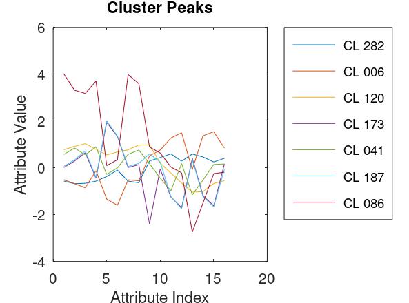
Unlike the frog call data set, where each attribute is MFCC value, the attributes of the bean data set contain various measures, including lengths, areas, and shape parameters, and had significantly different ranges. Therefore I decided to scale the attributes so that each had a mean value of zero and a standard deviation of one. Thus each attribute contributes equally to the distance metric. As with the frog data, I made a few runs with different threshold radii and settled on a similar result. The histogram and a scatter plot are shown here. Also shown, a plot of the attributes of the top 95 orphans.
The data set also included the actual bean type of each observation, so I was again able to tabulate the contents of the top 95 clusters. Although there is a perfect relation between the Bombay beans and cluster 086, the rest of the table is a mixed bag.
| Bean Type | CL 282 | CL 006 | CL 120 | CL 173 | CL 041 | CL 187 | CL 086 | |
| BARBUNYA | 130 | 5 | 276 | 0 | 851 | 5 | 0 | |
| BOMBAY | 0 | 0 | 0 | 0 | 0 | 0 | 333 | |
| CALI | 65 | 2 | 1523 | 6 | 2 | 8 | 0 | |
| DERMASON | 3442 | 62 | 0 | 0 | 0 | 0 | 0 | |
| HOROZ | 91 | 0 | 49 | 985 | 0 | 659 | 0 | |
| SEKER | 208 | 1797 | 0 | 0 | 3 | 0 | 0 | |
| SIRA | 2583 | 12 | 6 | 14 | 3 | 4 | 0 |
Table Analysis By Bean Type:
- Barbunya - mostly three-way split among clusters 282, 120, and 041
- Bombay - exclusively cluster 086
- Cali - mostly in cluster 120
- Dermason - mostly in cluster 282
- Horoz - mostly two-way split between clusters 173 and 187
- Seker - mostly in cluster 006, but many in cluster 282
- Sira - mostly in cluster 282
- Cluster 282 - mostly Dermason and Sira, but some of all but Bombay
- Cluster 006 - mostly Seker
- Cluster 120 - mostly Cali
- Cluster 173 - mostly Horoz
- Cluster 041 - mostly Barbunya
- Cluster 187 - mostly Horoz
- Cluster 086 - all Bombay

